10. Basics of recurrence relations#
In earlier units, we counted configurations directly using the sum, product, difference, and division rules, or packaged an entire sequence of counts into an ordinary generating function. For many combinatorial problems, however, an explicit formula is not immediately apparent either because a closed formula does not exist or
because it is not obvious how to derive it. Expressing the counts in terms of recurrence relations, when quantities associated to larger values of
Consider counting the ordered ways to write a positive integer
Instead of constructing every list of size
After studying these notes, you will be able to do the following.
Derive a recurrence relation by decomposing a set of combinatorial objects into mutually exclusive cases.
Identify the order of a recurrence, specify its required initial conditions, and determine its valid index range.
Classify a recurrence as linear or nonlinear, constant-coefficient or variable-coefficient, and homogeneous or nonhomogeneous.
Convert a constant-coefficient linear recurrence into an algebraic equation for its ordinary generating function, accounting for initial conditions.
Extract the recurrence relation and initial values satisfied by the sequence of coefficients of a rational generating function.
Model combinatorial structures such as: ordered compositions, pattern-avoiding strings, and restricted walks using recurrences and auxiliary state sequences.
10.1 Decomposing ordered sums into smaller subproblems#
Let
For small values of
To determine
Case 1: The list ends in
. A list in this case has the form . Removing the trailing leaves , which is an ordered list of s and s with sum . Conversely, appending to any ordered list with sum produces a valid list of sum ending in . Because removing the trailing and appending are mutual inverses, lists of sum ending in are in bijection with lists of sum . There are exactly such lists. Case 2: The list ends in
. A list in this case has the form . Removing the trailing leaves , which is an ordered list of s and s with sum . Conversely, appending to any ordered list with sum produces a valid list of sum ending in . These two operations are mutual inverses, so lists of sum ending in are in bijection with lists of sum . There are exactly such lists.
Every valid list belongs to exactly one of these two cases because its final entry is either
Starting from
| Final part | Ordered lists with sum | Count |
|---|---|---|
Thus
Notice why the condition
Together with
The same idea applies when more part sizes are allowed.
Let
For
How many ways can a
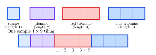
Solution:
The initial values are
10.2 Recurrences, order, and initial conditions#
A recurrence relation is a propagation rule for continuing a sequence. By itself, the rule does not identify a unique sequence; starting values are an indispensable part of the definition.
A complete recurrence relation of order
The order measures how far into the past the recurrence reaches. For instance, the recurrence
Consider the order-
With
and , we obtain the shifted Fibonacci numbers: With
and , we obtain the numbers (they have a name: "Lucas numbers"): With
and , every term is zero: .
The recurrence provides the propagation mechanism, the initial conditions anchor the sequence.
For the recurrences studied in this unit, three structural properties describe the form of the equation.
An order-
It has constant coefficients if each coefficient is a constant number
independent of , with . It is homogeneous if
for all . It is nonhomogeneous (or inhomogeneous) if
is not identically zero. The function is called the driving term or inhomogeneous term.
We classify each of the following recurrences by its order, linearity, coefficient type, and homogeneity:
: linear, order , constant coefficients ( ), homogeneous. : linear, order , constant coefficients, nonhomogeneous with driving term . : linear, order , variable coefficients (since depends on ), homogeneous. : linear, order , constant coefficients ( ), homogeneous. : nonlinear of order , because the earlier sequence terms and are multiplied together. : nonlinear recurrence of variable order, as seen for the Catalan numbers in Unit 2.
An equation alone does not define a sequence.
Consider the relation
With initial conditions
and , the sequence is constant: With initial conditions
and , the sequence grows linearly: If only
is specified, the term cannot be evaluated because is undetermined. An order- recurrence cannot begin without two initial values.
Similarly, the valid range of indices is essential. Applying
10.3 From a recurrence to an ordinary generating function#
Let
10.3.1 The procedure for second-order recurrences#
To understand how the algebra works, consider an order-
Multiply and sum over the valid index range. Multiply the recurrence by
and sum over all indices where the recurrence holds: Express each sum in terms of
. The sum on the left-hand side is missing the first two terms of : For the first sum on the right-hand side, factor out to align the exponent of with the index of : For the second sum, factor out : Substituting these three representations back into the summed recurrence gives Collect
and solve. Move all terms containing to the left-hand side and all initial condition terms to the right-hand side: Dividing by yields the generating function:
Notice the structure of the result:
The denominator
is determined entirely by the recurrence relation. The numerator
is determined by the initial conditions.
Let
10.3.2 The general order-
The same three-step procedure applies to linear recurrences of any finite order
Let
Multiply the recurrence by
If the recurrence in Theorem 10.8 is homogeneous, then
A frequent student error when converting an order-
Let
Solution:
Find the denominator. Here
, , and , so the theorem gives Fit the initial polynomial to the initial data. Because the recurrence is homogeneous, the theorem gives
Equivalently, Using only the coefficients through degree , Therefore,
10.4 From a rational generating function to a recurrence#
We can also read the connection between rational generating functions and recurrences in reverse. Multiplying a rational generating function by its denominator produces a polynomial, whose coefficients must eventually vanish.
Suppose the ordinary generating function of a sequence
Apply Theorem 10.8 in reverse. Multiplying by the denominator gives
The condition
Consider the rational generating function
Solution:
Find the recurrence and its valid range. Write the denominator in the standard form
Thus , , and the recurrence has order . Since the numerator has degree , Proposition 10.11 applies at every : Find the initial conditions. Use the identity
Equating the coefficients of and gives Therefore and .
Using the recurrence
As an independent check, we can expand
10.5 Pattern-avoiding strings#
A string over an alphabet 0010 contains 00 in its first two positions and therefore does not avoid 00.
Pattern avoidance is a global condition, not merely a restriction on how a string ends. The string 0011 ends in 11, but it contains 00 at its start, so it fails to avoid 00.
10.5.1 Binary strings avoiding repeated zeroes#
Let 00.
For
, the empty string contains no characters and vacuously avoids 00, so. For
, both length- strings 0and1avoid00, so.
For 1 or 0.
Case 1: The string ends in
1. A string in this case has the form. Because the added final character is 1, it cannot complete a forbidden block00. Therefore,avoids 00if and only if the prefixavoids 00. There aresuch strings. Case 2: The string ends in
0. Becauseand the string avoids 00, the character immediately preceding the final0cannot be0. It must be1. Thus, every valid string ending in0actually ends in the two-character block10:Because the block 10begins with1, appending it to any valid string of lengthcannot create 00. Therefore,avoids 00if and only if the prefixavoids 00. There aresuch strings.
Because every valid string ends in either 1 or 0, the two cases partition the set of valid strings:
00 is forbidden, leaving 01, 10, 11, which confirms
Using our generating function formula for order-
Let 000.
For 000, so
10.5.2 A nonhomogeneous recurrence: avoiding one-zero#
Let 10.
In any valid string, once a 1 appears, every subsequent character must also be 1; a 0 appearing anywhere after a 1 would create a 10 transition. Every valid string therefore consists of
We can also derive this result by setting up a recurrence based on the final character:
For
If the string ends in
1, removing that1leaves an arbitrary valid string of length. (Appending 1can never create10). This yieldsstrings. If the string ends in
0, it cannot contain a1in any earlier position, because any earlier1followed eventually by this final0would require at least one10transition. Thus, all precedingcharacters must be 0. This yields exactlystring: .
Because these two cases are disjoint and cover all valid strings, we obtain
We convert it to a generating function using Theorem 10.8. Multiply by
10.5.3 Alphabet size and subtraction techniques#
When the alphabet contains more than two symbols, the number of choices for allowed final characters scales the recurrence coefficients.
Let 00.
For
For
If it ends in
1or2: the preceding prefix can be any valid string of length. There are choices for the final symbol, contributing strings. If it ends in
0: the preceding symbol cannot be0, so it must be1or2. The string ends in10or20. The prefix of lengthcan be any valid string. There are choices for the block, contributing strings.
Combining the cases:
00 is forbidden).
The generating function is
The difference rule from Unit 1 is particularly effective when an allowed ending is described by subtracting an exception from all valid prefixes.
Let 10.
For
For
If the final symbol is
1or2: appending1or2to any valid length-string can never create 10. This producesvalid strings. If the final symbol is
0: we may append0to any valid length-prefix except those that end in 1. How many valid length-strings end in 1? A valid string of lengthending in 1is formed uniquely by appending1to an arbitrary valid string of length. (Appending 1never introduces10). Thus, exactlyof the valid prefixes end in 1. By the difference rule, the number of valid prefixes that do not end in1is.
Summing the allowed endings:
10 is forbidden, leaving 10 (100, 101, 102, 010, 110, 210), leaving
The generating function has denominator
10.6 Walks with forbidden reversals: a lucky simplification#
Suppose a robot moves on the integer lattice LR and RL are forbidden. Let
To extend a valid walk of length
If it ends in
U, all three next steps are allowed.If it ends in
LorR, exactly two next steps are allowed.
Let U. The remaining U to any valid walk of length U, and removing the final U reverses this operation. Therefore,
The sequence begins
LR and RL are forbidden, confirming
The generating function has denominator U—are in immediate bijection with all valid walks one step shorter. For more complicated local restrictions, each ending type may have its own continuation rules, and no exceptional count collapses so neatly to an earlier total. We will need a reliable method, based on state variables and matrix recurrence relations, to model that more difficult logic.
10.7 Boundary choices: decomposing from the start versus the end#
In the examples developed so far, we decomposed objects by examining their final element—the last part of a sum, the trailing symbol of a string, or the final step of a walk. Decomposing by the first element is equally valid and can sometimes simplify the argument.
10.7.1 Initial character decomposition in pattern avoidance#
Consider again the sequence 10 from Section 10.5.2. When we decomposed by the final character, strings ending in 0 required an argument showing that all previous symbols had to be 0.
Let us instead classify a valid string of length
Case 1: The string begins with
0. Prepending0to any valid string of lengthcannot create 10, because the newly added character is0. Therefore, any valid string of lengthcan serve as the suffix. This yields strings. Case 2: The string begins with
1. If the string begins with1, it can never contain a0in any subsequent position, because a0anywhere after this leading1would create a10transition. Thus, all remainingcharacters must be 1. This yields exactlystring: .
Because every valid string begins with either 0 or 1, the sum rule immediately reproduces
10.7.2 A geometric model: tiling a grid with dominoes#
Decomposing from a boundary is also the fundamental tool for counting tilings of two-dimensional regions.
How many ways are there to tile a
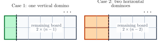
Solution:
Let
For
Case 1: The top-left square is covered by a vertical domino. A vertical domino occupies both squares of column
(row and row ). Removing this domino leaves an uncovered board. Conversely, placing a vertical domino in column next to any valid tiling of a board produces a valid tiling of the board. Thus, there are tilings in this case. Case 2: The top-left square is covered by a horizontal domino. A horizontal domino occupies the top squares of columns
and . Now consider the bottom square of column (row , column ). It cannot be covered by a vertical domino, because the square above it is already occupied. It cannot be left empty. Therefore, it must be covered by another horizontal domino, which occupies the bottom squares of columns and . Together, these two horizontal dominoes completely fill columns and , forming a block. Removing both horizontal dominoes leaves an uncovered board. Conversely, placing two horizontal dominoes in the first two columns next to any valid tiling of a board produces a valid tiling of the board. Thus, there are tilings in this case.
Every valid tiling covers the top-left square in exactly one of these two ways, and the two cases leave independent sub-boards. The sum rule therefore gives
The domino tiling problem demonstrates that whether objects are represented as algebraic lists, character strings, or geometric tiles, the underlying combinatorial technique is identical:
Isolate an indispensable boundary element (such as the final part, first symbol, or a fixed corner square).
Classify the mutually exclusive ways to cover or choose that boundary element.
Establish bijections between each case and smaller instances of the original problem to determine the recurrence relation and initial conditions.
10.8 Two next questions#
Now that we covered the basics of recurrence relations, we still need to understand two questions.
How do we solve the recurrence?
How do we model more complex recurrence problems?
Let
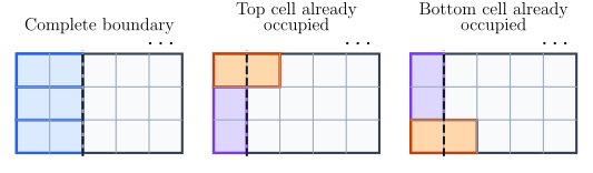
The pictures show the obstacle. After removing tiles near the left boundary, the remaining region may be a smaller complete rectangle, but it may instead have a top or bottom boundary square already occupied by a horizontal domino. The number
Consequently, a recurrence involving only the totals
Let
This recurrence is difficult to guess from the totals abc, bca, and cab forbid different next letters. These suffixes also overlap—the ending of one nearly forbidden pattern can be the beginning of another. A reliable model therefore needs states recording the longest relevant suffix of the current string, rather than only the total number of valid strings.